It is officially the end of my internship at Deezer and I am back to a Sunny and extremely humid Barcelona. Locked in my room with the fan running at insane speed I am going to reminisce about the work I did for the last 3 months.
My research was exploring Embedding aggregation and strategies for use in Recommendations systems. At the core of all of this is the relationship between tracks, which is defined using Playlists. We build this using a simple Co-Occurrence matrix, which is quite sparse so its followed by Singular Value Decomposition which is essentially just a dimensionality reduction technique to generate dense, low dimensional embeddings.
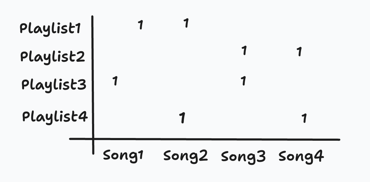
Once we have track embeddings, we can perform aggregations on these embeddings, and this aggregation can help us represent higher level abstractions like Artists, Albums and Genres. The standard way is to average the embeddings but existing work done with this paper empirically proves that real-world averages are less consistent for recommendation.
The work started here with the definition of what makes a “Good centroid”, I went about defining this using two metrics:
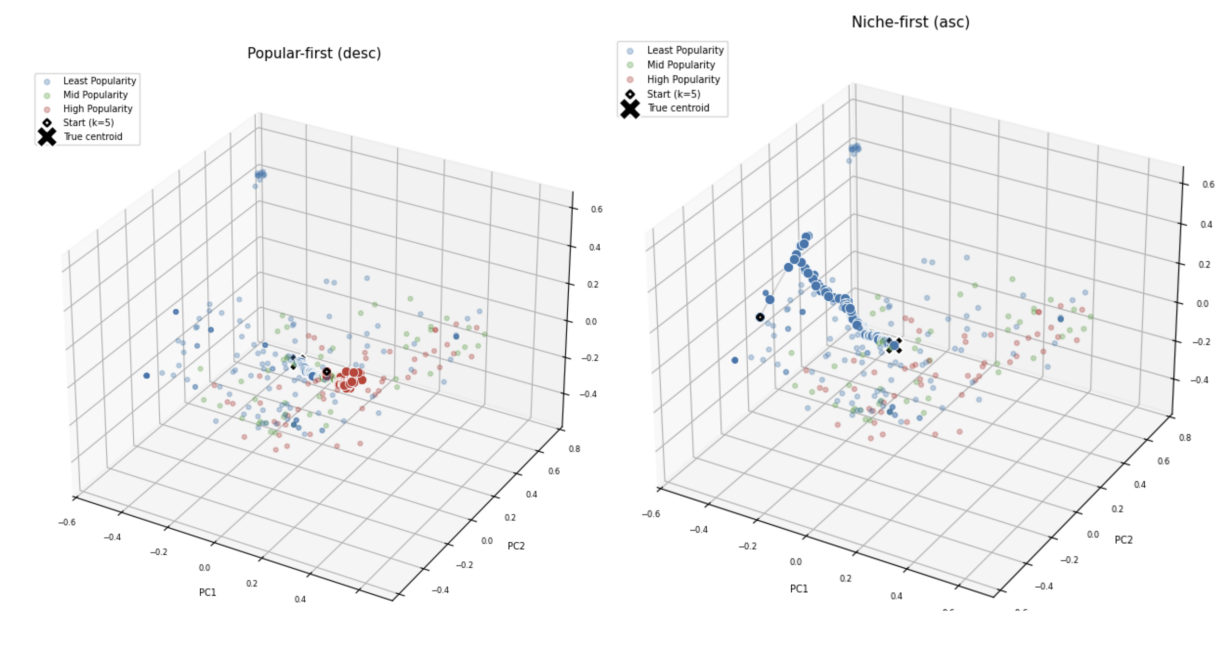
Stability: How much the centroid shifts as we keep adding more tracks?
This metrics is really dependent on the popularity of the tracks and reveals things about the embeddings structure
- Centroids moves around a lot for niche tracks.
- For popular tracks move around the least.
- The consistency lies in the middle when we randomly sample tracks.
But in the end, centroids converge after ~20 track which means they stop moving around and stabilize BUT at different rates, so we can literally see the long tail (it do be long)
Consistency: What percentage of entity belong to the top K neighbors from the centroid?
Rather than choosing entities at random we look around the centroid of an entity i.e an artist and fetch the K nearest tracks and check what percentage of those K tracks actually belong to the artist.
Aligning with what the paper establishes, this metric goes down as we increase the number of K. When we order the tracks and choose K by popularity then the consistency metric improves, highlighting the findings from stability but still has a downward trend.
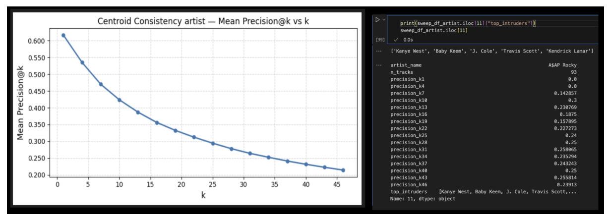
We already know SVD has a popularity bias but this plays a big part in aggregation cause now centroids start to make more sense only for popular tracks.
A way to tackle this would be to inject concept information i.e artist, album into our SVD, How?
Higher Order SVD
The intuition is simple, rather than factorizing just the track playlist co-occurrence we add an additional entity, for example: track artist co-occurrence and factorize with this added dimension. This becomes a tensor factorization. There are several ways to decompose this tensor, the specific method I ended up using is Tucker decomposition.
This pulls the concepts closer to each other while still maintaining the semantics of track playlist co occurrence, we can also control how much of this dimensionality we should add
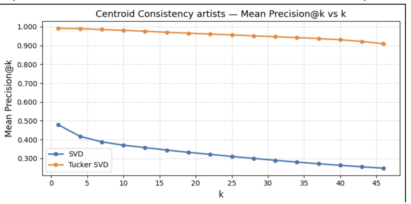
This drastically increases the consistency metric and inverts the stability metrics. Now the popular tracks leave a long trail cause they got pulled away from it’s co-occurrence bubble.
But the actual metrics that we use to evaluate these embeddings fail because they are meant to recreate the co-occurrence and by adding a new dimension we cheated and broke it.
An interesting observation while evaluating these HO-SVD embeddings was that, on real user streaming data, Artist aligned embeddings consistently outperform in most listening contexts, which means that real user listening habits tend to be more artist aligned.
The normal SVD still performs good at the traditional recommendation metrics like NDCG because they are all based on playlist reconstruction but now that the embeddings have been pulled apart we would need to evaluate it different, I tried intrinsic evaluation metrics based on the geometry of the embeddings i.e how feature vectors are distributed across a latent space. A high-quality embedding space typically balances alignment (similar items group together) and isotropy (data utilizes the full vector space rather than collapsing).
- Shannon Entropy: Evaluates the spread of variance across dimensions
- Effective Rank: Number of dimensions being utilized (Global/ Local)
Global is calculated across the entire dataset whereas Local is within small, localized neighborhoods.
These experiments with Geometry made me discover Hyperbolic space and that led to some further work.
Hyperbolic Space
In complex networks (like our track playlist interactions), data often follows power law. This means that a very small number of items are exceptionally popular (the head), while a massive number of items are rarely interacted with (the long tail)
When we model song-playlist co-occurrences in Euclidean space we lose information especially since there is already an inherent hierarchy in the data and as this hierarchy expands exponentially, Euclidean embeddings require increasing distortion, leading to information loss and poor preservation of relationships. Hyperbolic space, with its constant negative curvature, naturally accommodates this exponential growth, enabling low-distortion embeddings that preserve both local and global hierarchical structure.
I trained a simple Hyperbolic Autoencoder on a Poincaré ball using HypTorch on the PPMI matrix calculated from the co-occurrence.
Straight away I notice that Hyperbolic model builds a negative correlation with the rank of the track, so popularity tends to grow radially outwards.
Running a linear probing experiment for evaluation: For each embedding space, we run PCA per principal component (or per block of 5-10) and train a simple linear probe to predict entities like artist and genres across the different embeddings, And I notice that the hyperbolic model is capable to disentangling these clusters better than the normalised SVD and we do not need so many dimensions (128) in Hyperbolic dimension to encode as much information as in an Euclidean space.
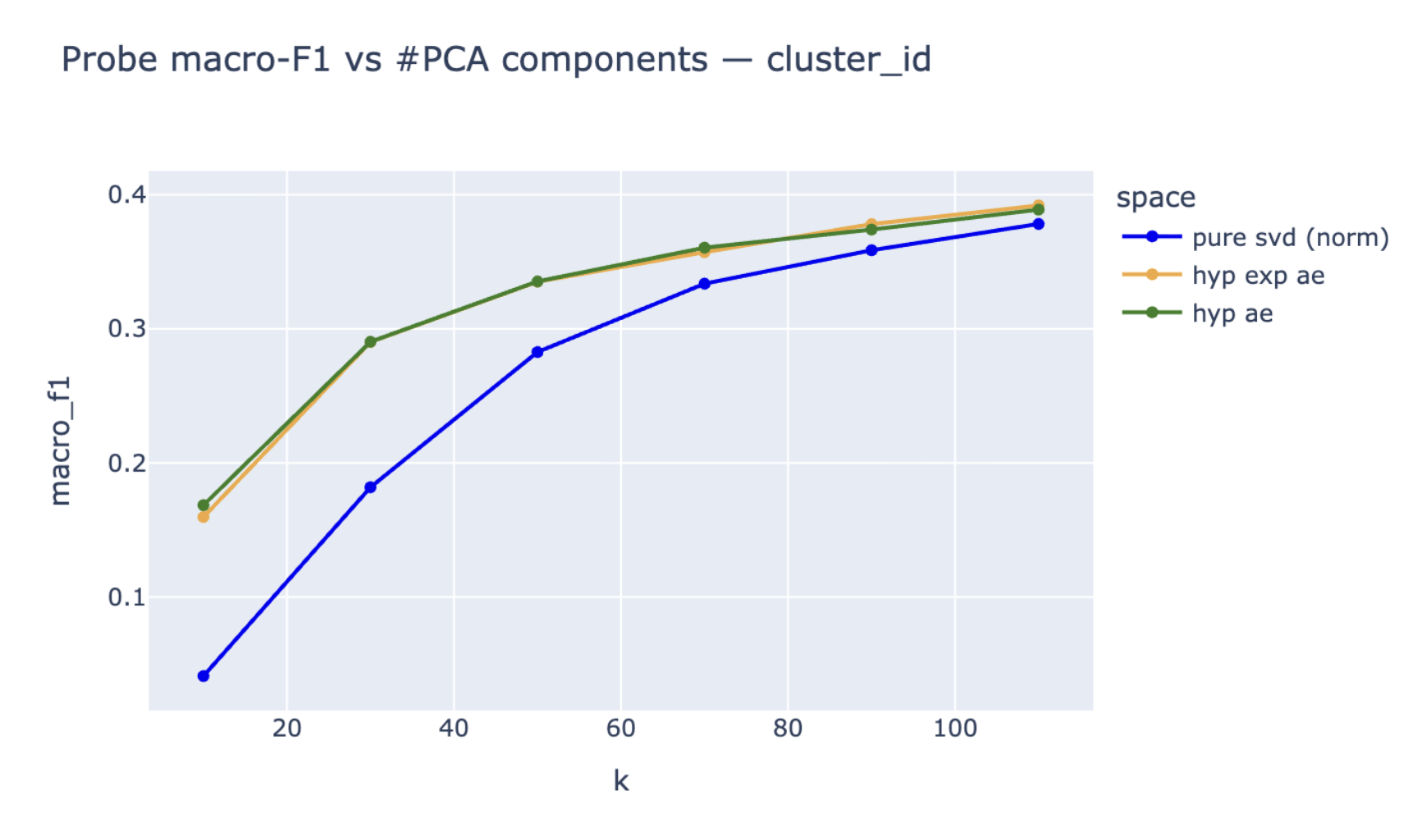
Geometrically, looking at the Isotropy: SVD has the highest global effective rank because of Spiky SVDs but also the lowest local rank whereas Hyperbolic space manages to maintain a high global and local rank.
This is just a short description of what I did, not really an official report with the metrics, Some interesting experiments that I noted down for the future
- Run Interpretability experiments with Visualization on Hyperbolic space
- Explicitly inject hierarchical information is the loss function (Genre, Artist, Album) right now hyperbolic space loss just recreates the track-playlist PPMI
I do have these experiments reproduced on Spotify 1M Playlists dataset but the code is not public but I hope to clean it up soon.
Leave a Comment