Variational Autoencoders for Audio

A major division in machine learning is generative versus discriminative modeling. While in discriminative modeling one aims to learn a predictor given the observations, in generative modeling one aims to solve the more general problem of learning a joint distribution over all the variables.

As a hater of AI music, Why should I care About Generative Models? Well, when used right, they are pretty good tools.

Scientific Understanding: When meteorologists model weather, they don’t just predict “rain or shine.” They model the underlying physics - pressure systems, temperature gradients, moisture flows. That’s generative modeling!
Causal Relations: Generative models naturally express cause and effect. Understanding the generative process of earthquakes helps us use it anywhere in the world.
Data Efficiency: When you have few labeled examples but lots of unlabeled data, generative models can help. They learn the structure of the data itself, not just decision boundaries.

How can we do this type of modeling?

Directed Graphical Models

Directed graphical models, also known as Bayesian networks or directed acyclic graphs (DAGs), are probabilistic graphical models that represent a set of random variables and their conditional dependencies using a directed acyclic graph structure.

The probability of everything happening equals the product of each thing happening given its “parents” (causes). We can use neural networks to parameterize these conditional distributions and get representations of arbitrarily complex functions.

This gives us the expressive power to model real-world data like images and audio!

We just talked about modeling relationships between things we can observe. But most of what determines our observations is hidden from us, and these are called Latent Variables (z).

p(x) = ∫ p(x|z)p(z) dz

This integral is saying:

The probability of seeing data x equals the sum over all possible hidden explanations z, weighted by how likely each explanation is

Sampling latent variables z from a simple distribution might give us z₁ that can maybe represent genres, and once we pass z through a neural network, we can transform these abstract numbers into values that can model the genre of the audio. What is cool about these variables is that they are:

Continuous: Smoothly interpolate across genres
Disentangled: Different dimensions control different aspects
Compact: Complex audio features reduced to few numbers

Here’s where it gets a bit tricky. To train our DLVM (Deep Latent Variable Models), we need to maximize the likelihood of our training data

log p(x) = log ∫ p(x|z)p(z) dz

But this integral is intractable because we have to do high-dimensional integration! lmao, I can’t even integrate well in the current dimension and if z has 100 dimensions, we’re integrating over a 100-dimensional space. Good luck with that brother.

Even worse, to train the model, we need to know the posterior distribution p(z|x). if that sounded like nonsense, It means that given an audio file, we need to predict the likely latent factors that generated it? and by Bayes’ rule:

p(z|x) = p(x|z)p(z) / p(x)

But we just said p(x) is intractable, so p(z|x) is also intractable.

What do we do now?

VAE (Amortized Variational Inference)

There is always a way! The basic idea is this: If we can’t compute the true posterior p(z|x), let’s approximate it! But traditional variational inference optimizes a separate approximate posterior for each data point. If you have a million audio files, you need a million separate optimizations. This is impossibly slow!

So we can simply Use a neural network to predict the posterior for ANY input

This is called “amortized” inference because we share (amortize) the computational cost across all data points. A VAE introduces an “inference network” or “encoder” that approximates the true posterior.

VM Functions

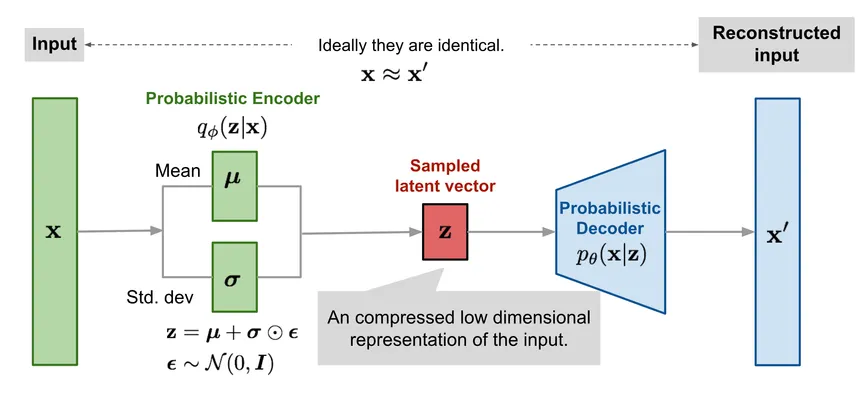
A VAE consists of two neural networks:

Encoder (Inference Network):

Input: Observation x (e.g., an audio file)
Output: Distribution parameters for z (typically mean μ and variance σ²)
Learns to infer latent factors from observations

Decoder (Generative Network):

Input: Latent code z
Output: Distribution parameters for x (e.g., pixel means)
Learns to generate observations from latent factors

Together, they form a probabilistic autoencoder!

Unlike deterministic autoencoders, VAEs model the latent space as a probability distribution. This produces a probability distribution function over the input encodings instead of just a single fixed vector. This allows for a more nuanced representation of uncertainty in the data. The decoder then samples from this probability distribution.

The latent space in VAEs serves as a continuous, structured representation of the input data. Since it is continuous by design, this allows for easy interpolation. Each point in the latent space corresponds to a potential output, enabling smooth transitions between different data points and also ensuring that points which are closer in the latent space lead to similar generations.

ELBO

Let’s start with what we actually want to maximize: the log probability of our data

log p(x) = log probability that our model generates x

As discussed, we can’t compute log p(x) directly, but we can compute a lower bound that we can optimize to get closer to p(x). Technically, when ELBO equals log p(x), we’ve found the perfect model!

log p(x) ≥ ELBO

ELBO tells us what to optimize, but we have a major issue with training our encoder. Since we need randomness in our model to train the VAE, when running backpropagation we can’t meaningfully update parameters based on random outcomes.

Backpropagation requires the ability to compute exact gradients and since the sampling operation is random, it doesn’t have a well-defined gradient.

We cannot learn anything from sampling random values, So we use a reparameterization trick which just changes what we’re learning (respond to randomness instead of sampling randomness itself)

# Split into: fixed randomness + learned response
ε = sample_random_number()  # Fixed randomness (like wind)
z = μ + σ × ε              # Learned response to randomness

The reparameterization trick works by separating the deterministic and the stochastic parts of the sampling operation. Instead of directly sampling from the distribution we sample epsilon from a standard normal distribution and compute the desired sample z as:

z = mu + sigma * epsilon

Here epsilon introduces the necessary randomness The operation mu + sigma * epsilon is entirely deterministic and differentiable, meaning we can apply backpropagation through it. This method allows us to incorporate the random element required for sampling from the latent distribution while preserving the chain of differentiable operations needed for backpropagation.

This is the python method

def reparameterize(self, mu, log_var):
    """
    Reparameterization trick: z = mu + sigma * epsilon
    where epsilon ~ N(0, 1)
    """
    if self.training:
        # Sample noise
        # Convert log variance to standard deviation
        std = torch.exp(0.5 * log_var)
        eps = torch.randn_like(std)
        return mu + eps * std
    else:
        # During evaluation, just return the mean
        return mu

Epsilon with its randomness reflects the probabilistic nature of the latent space that we’re trying to model

The combination of ELBO and the reparameterization trick helps us create a tractable objective for an intractable problem and makes that objective differentiable so we can train generative models with gradient descent.

The loss function for VAEs comprises two components:

Reconstruction loss (measuring how well the model reconstructs the input) similar to the vanilla autoencoders
KL divergence (measuring how closely the learned distribution resembles a chosen prior distribution, usually gaussian).

The combination of these components encourages the model to learn a latent representation that captures both the data distribution and the specified prior.

def elbo_loss(x_recon, x, mu, log_var, beta=1.0):
    batch_size = x.size(0)
    
    # Negative log-likelihood (Gaussian decoder with unit variance)
    recon_loss = 0.5 * F.mse_loss(
        x_recon, x, reduction='sum'
    ) / batch_size

    # KL divergence
    # Sum over latent dimensions, mean over batch
    kl_loss = -0.5 * torch.sum(
        1 + log_var - mu.pow(2) - log_var.exp()
    ) / batch_size

    # We return negative ELBO as the loss to minimize
    elbo = -recon_loss - kl_loss
    neg_elbo = recon_loss + beta * kl_loss

    return neg_elbo, recon_loss, kl_loss, elbo

In PyTorch, the ELBO loss can be implemented by combining a reconstruction loss function, such as binary cross-entropy with the KL divergence term. The total loss is then minimized using an optimizer like Adam.

Incorporating the KL divergence term into the loss function, VAEs are encouraged to learn a latent space where similar data points are closer, ensuring a meaningful and structured representation. The autoencoders loss function aims to minimize both the reconstruction loss and the latent loss. A smaller latent loss implies a limited encoding of information that would otherwise enhance the reconstruction loss. Consequently, the VAE finds itself in a delicate balance between the latent loss and the reconstruction loss.

This equilibrium becomes pivotal, as a smaller latent loss tends to result in generated audio closely resembling those present in the training set but lacking in visual quality.

Conversely, a smaller reconstruction loss leads to well-reconstructed audio during training but hampers the generation of novel audio that deviate significantly from the training set. Striking a balance between these two aspects becomes imperative to achieve desirable outcomes in both image reconstruction and generation.

A really cool model that uses VAEs to have both fast and high-quality audio waveform synthesis is RAVE

I have implemented a simple VAE using the MagnatagATune dataset and when I initially started training I faced this issue

Annealing

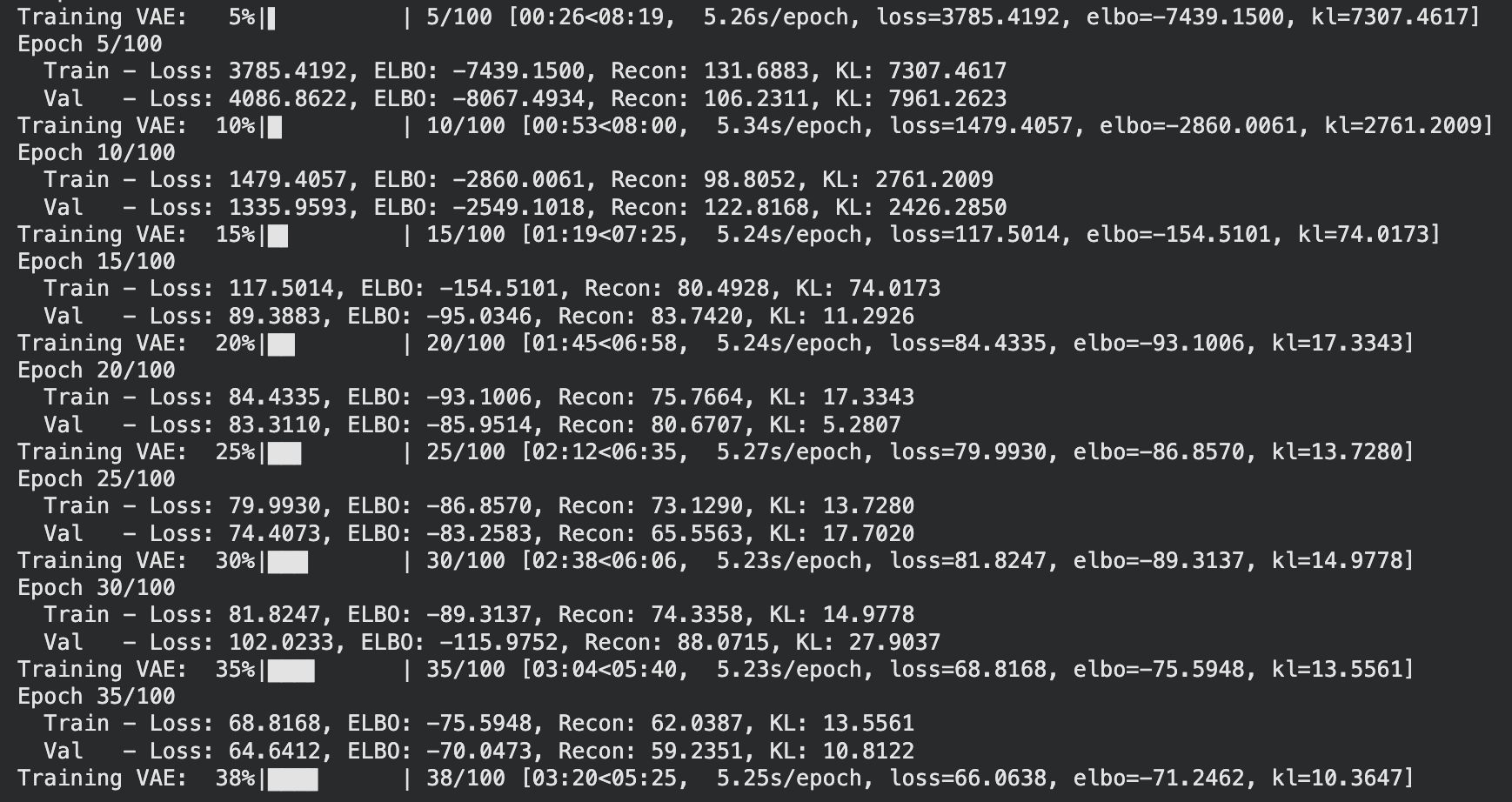
KL is collapsing (7307 → 74 → 11), this is called the KL vanishing problem and a solution is Cyclical annealing, which is basically repeatedly increasing the weighting hyper-parameter that controls the strength of the KL regularization in multiple cycles

I have uploaded down the code for this VAE and all the subsequent experimentation here: 📓 Open in Colab

Variational Autoencoders for Audio

Directed Graphical Models

VAE (Amortized Variational Inference)

Encoder (Inference Network):

Decoder (Generative Network):

ELBO

Links

Comments

Leave a Comment

FEATURED TAGS