I haven’t seen the original 1982 TRON, but I just saw the trailer and it looks hilarious. It was the first film to use computer-generated imagery extensively and was considered avant-garde at the time, so it makes sense I find it funny now because we’re so used to hearing about CGI in movies these days. It’s no longer new, and now there are a ton of AI tools that can be used to manifest worlds while sitting at home typing prompts. As hilarious as the poster looks, TRON did inspire a generation of computer nerds in the 80s.
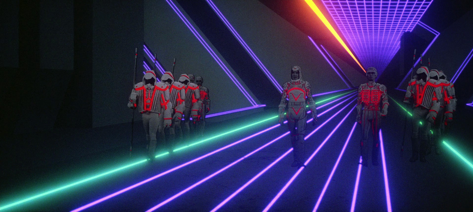
The cool image that you see above is built with mathematical primitives. The film did require meticulous manual calculations and mapping out movements individually because computer systems could only render still images, so a motion picture camera was placed in front of a computer screen to capture each individual frame. What’s crazier is that they did all of this with computers having 2 MB of memory and no more than 330 MB of storage.
Mad lads!!
Ken Perlin, a research scientist for Mathematical Applications Group at the time, was one of those mad lads roped in to work on special effects for the movie. While Ken enjoyed the work, he found himself frustrated with the “machine-like” look that existed due to the technologies being used.
At the time, they were using polygons to produce shapes, but Ken thought of textures in terms of volumes rather than flat surfaces. He realized that filling these volumes with controllably generated noise produced realistic, interesting, and believable effects and images. This can create shapes with smooth, natural-looking randomness unlike pure random noise (which is jagged). These should be the properties of such a noise function.
- SMOOTH: Nearby inputs give similar outputs
- CONTINUOUS: No sudden jumps or breaks
- DETERMINISTIC: Same input always gives same output
- BOUNDED: Output stays within predictable range
This Perlin noise, as it came to be known, turned out to be a magic brush for digital artists. With it, they could paint wood, marble, and clouds that looked real without storing a single image. By 1984, when Perlin presented it at SIGGRAPH, the graphics world quickly took notice. What started as his quest to break the plastic perfection of TRON-style graphics became one of the most important inventions in visual effects, so much so that it later earned him an Academy Award.
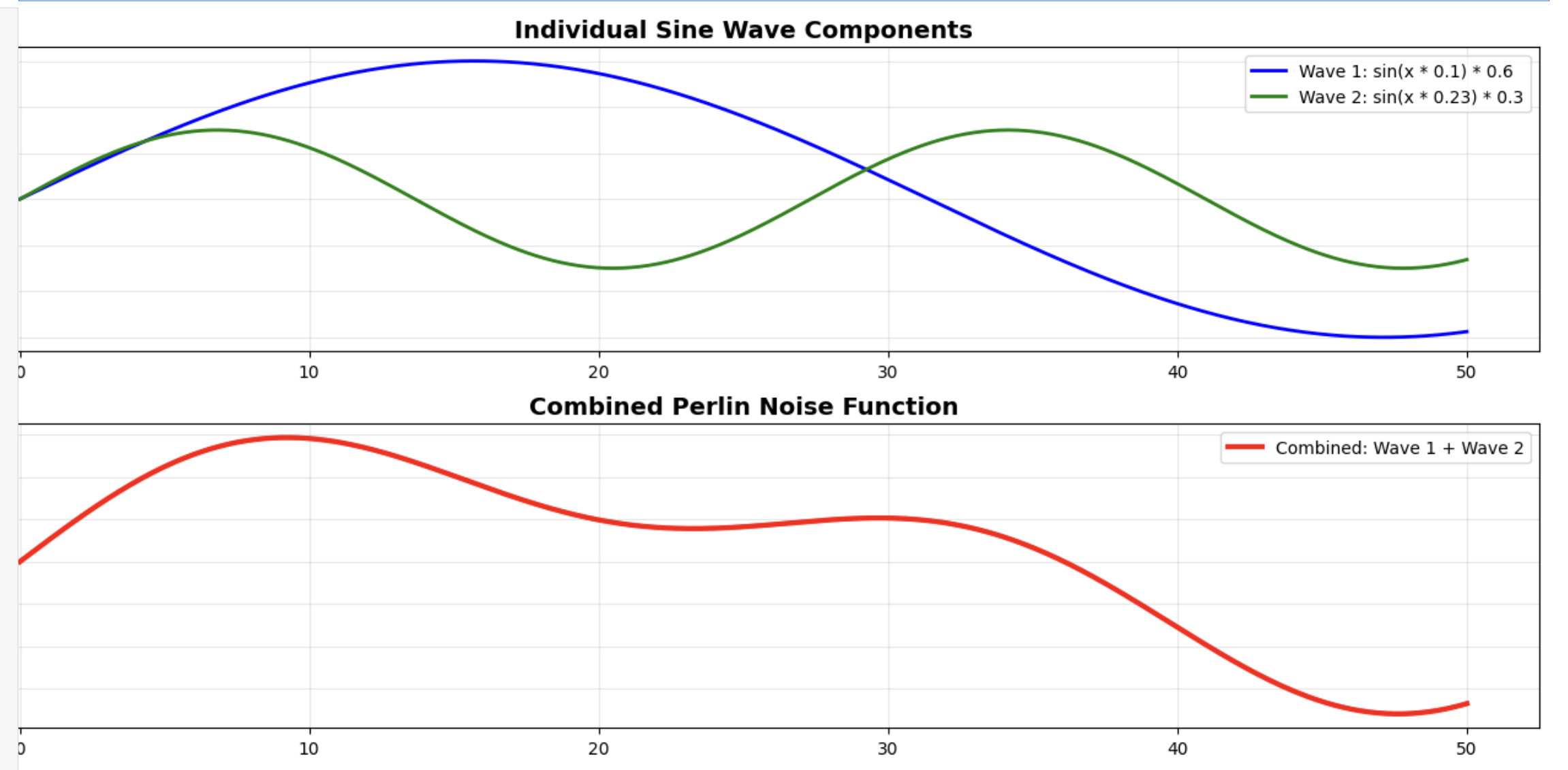
We can actually simulate its properties, although at a smaller level, using sine waves and Fourier synthesis with the core idea of using a sum of sine waves with varying frequencies and amplitudes to create complex, seemingly random patterns.
Let’s take these two waves as examples and combine them
wave1 = math.sin(x * 0.1) * 0.6  # Low frequency, high amplitude
wave2 = math.sin(x * 0.23) * 0.3  # Higher frequency, lower amplitude
simulated_noise = wave1 + wave2
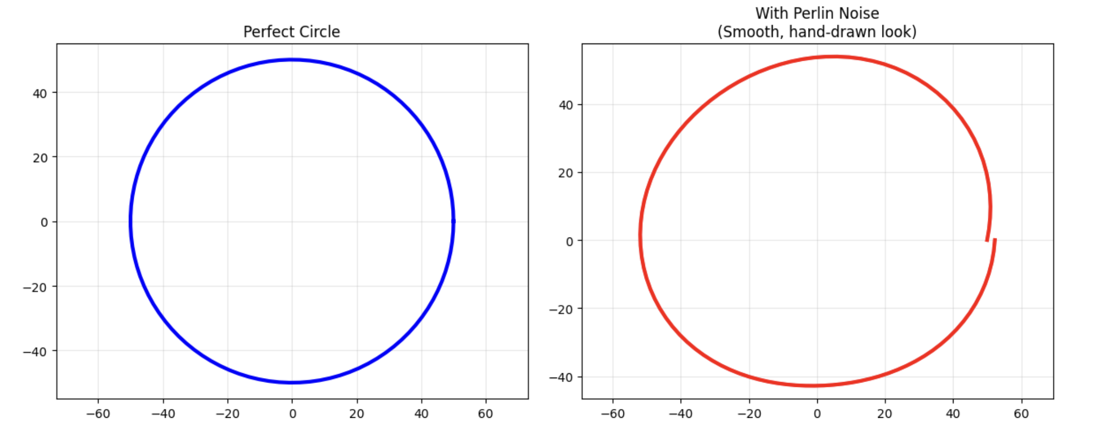
Here is a simple circle. We can add this noise to it by varying the radius using the angle as noise input. After scaling, we get a circle that looks hand-drawn rather than machine-generated, with imperfections.
# Generate circle points
angles = np.linspace(0, 2 * math.pi, 100)
radius = 50

# Perfect circle
perfect_x = [radius * math.cos(a) for a in angles]
perfect_y = [radius * math.sin(a) for a in angles]
And now let’s apply our noise function to it!
def noise(x):
    return math.sin(x * 0.1) * 0.6 + math.sin(x * 0.23) * 0.3

# Noisy circle
noisy_x = []
noisy_y = []
for a in angles:
    # Add noise to radius based on angle
    noisy_radius = radius + noise(a * 10) * 8  # Scale angle and noise
    noisy_x.append(noisy_radius * math.cos(a))
    noisy_y.append(noisy_radius * math.sin(a))
Plot these two circles:
# Plot both circles
plt.figure(figsize=(12, 5))

plt.subplot(1, 2, 1)
plt.plot(perfect_x, perfect_y, 'b-', linewidth=3)
plt.title('Perfect Circle')
plt.axis('equal')
plt.grid(True, alpha=0.3)

plt.subplot(1, 2, 2)
plt.plot(noisy_x, noisy_y, 'r-', linewidth=3)
plt.title('With Perlin Noise\n(Smooth, hand-drawn look)')
plt.axis('equal')
plt.grid(True, alpha=0.3)

plt.tight_layout()
plt.show()
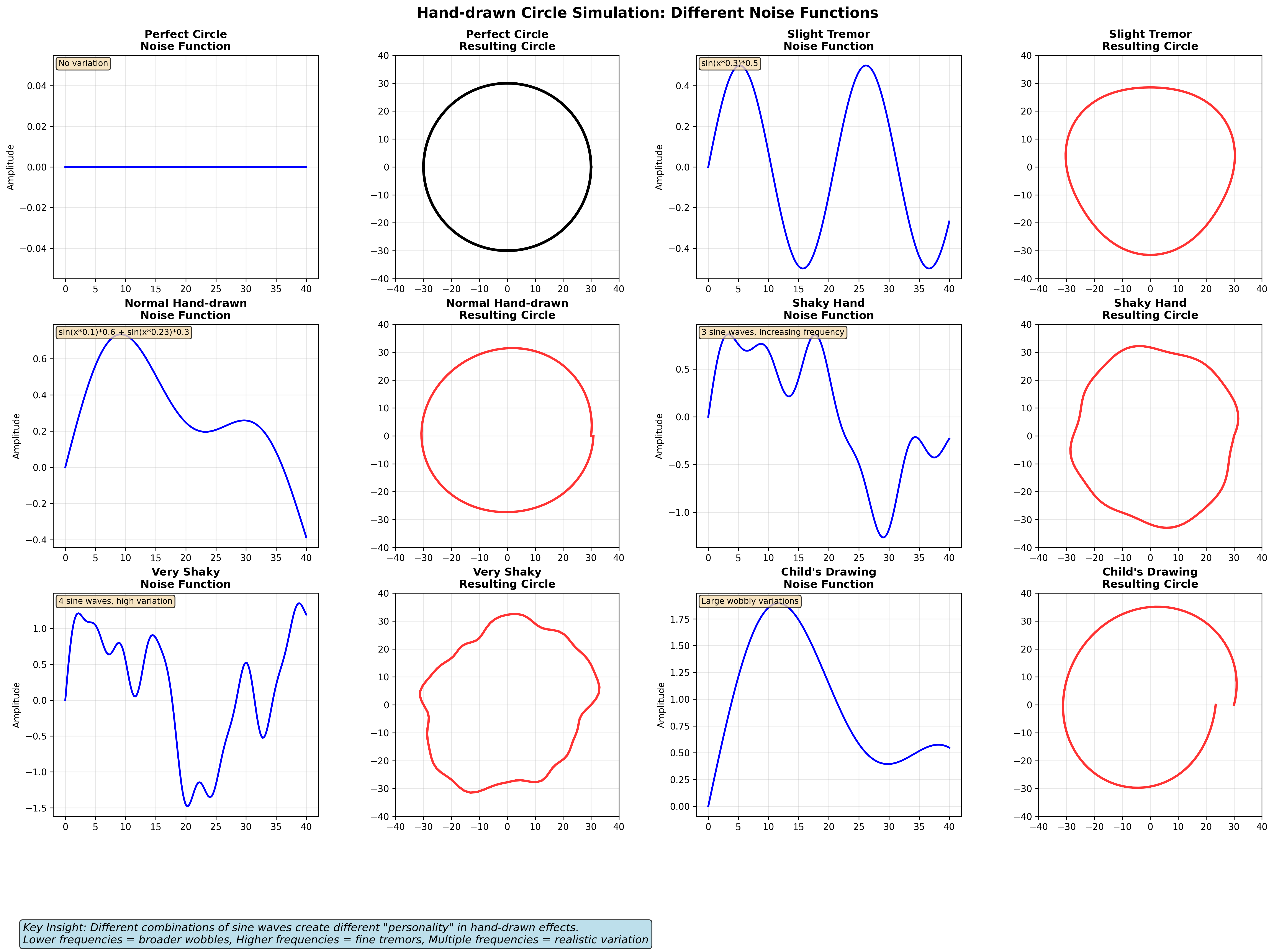
We can also simulate the same experiment with different sine wave combinations to get different degrees of noise in the output circle.
 Open in a new tab or zoom in
We just added multiple “layers” of noise together, each with a different amplitude and frequency, and when one layer has a frequency that is double the frequency of the previous layer, this layer is called an octave.
The example we saw was just for a single dimension, if you extend Perlin Noise into an additional dimension and consider the extra dimension as time, you can animate it! For example, 2D Perlin Noise can be interpreted as Terrain, but 3D noise can similarly be interpreted as undulating waves in an ocean scene.
Let’s now explore this concept with a 2-dimensional vector. Perlin noise isn’t just random values, it’s about directional influence. To calculate that, we can use the very handy dot product, and the other important idea here is interpolation, which becomes much more straightforward between 4 corners. So we start by
Setting up 2D Grid
We start by setting up a grid with a certain number of floating points, 2 for 2 dimensions (x,y). Now, x and y can be anything, but they are generally a position. To generate a texture, x and y would be the coordinates of the pixels in the texture (multiplied by the frequency).
class VectorGrid:
    """Simple 2D vector class for dot product calculations"""

    def __init__(self, x: float, y: float):
        self.x = x  # X component of the vector
        self.y = y  # Y component of the vector

    def dot(self, other: 'VectorGrid') -> float:
        """Calculate dot product with another vector"""
        return self.x * other.x + self.y * other.y

    def __repr__(self):
        return f"VectorGrid({self.x:.2f}, {self.y:.2f})"
Creating the Permutation Table
This is what makes Perlin noise deterministic. It’s basically an array containing numbers 0-256 (8-bit era) in shuffled order, used to assign consistent random vectors to grid points.
def shuffle_array(array_to_shuffle: List[int]) -> None:
    """Shuffle algorithm to randomize array in-place"""
    for i in range(len(array_to_shuffle) - 1, 0, -1):
        j = random.randint(0, i)
        # Swap elements at positions i and j
        array_to_shuffle[i], array_to_shuffle[j] = \
        array_to_shuffle[j], array_to_shuffle[i]

def make_permutation() -> List[int]:
    """Create the permutation table used by Perlin noise"""
    #  # [0, 1, 2, ..., 255]
    permutation = list(range(256))

    # Shuffle it to create random but deterministic order
    shuffle_array(permutation)
    permutation.extend(permutation)

    return permutation
This creates a sort of deterministic chaos where the permutation table acts as a memory system to assign gradient vectors to grid points. In 2D, we use one of 4 possible vectors: (1,1), (1,-1), (-1,-1), (-1,1). The permutation table determines which vector each grid point gets.
def get_constant_vector(v: int) -> VectorGrid:
    """Get gradient vectors based on permutation table value"""
    h = v & 3  # Equivalent to v % 4, gives us 0, 1, 2, or 3

    # Return one of 4 diagonal vectors based on h value
    if h == 0:
        return VectorGrid(1.0, 1.0)    # Northeast
    elif h == 1:
        return VectorGrid(-1.0, 1.0)   # Northwest
    elif h == 2:
        return VectorGrid(-1.0, -1.0)  # Southwest
    else:  # h == 3
        return VectorGrid(1.0, -1.0)   # Southeast
The permutation table acts like a memory to get consistent values for each grid corner, so the same grid point must always return the same value, regardless of which grid square we’re computing from.
Computing dot product
We calculate dot products between the corner-to-input vectors and the constant gradient vectors. This creates the smooth variation we want.
# Get constant gradient vectors for each corner
grad_tr = get_constant_vector(value_tr)
grad_tl = get_constant_vector(value_tl)
grad_br = get_constant_vector(value_br)
grad_bl = get_constant_vector(value_bl)

# Calculate dot products: corner_vector • gradient_vector
dot_top_right = top_right_vec.dot(grad_tr)
dot_top_left = top_left_vec.dot(grad_tl)
dot_bottom_right = bottom_right_vec.dot(grad_br)
dot_bottom_left = bottom_left_vec.dot(grad_bl)
Interpolation
Now that we have to dot product for each corner, we need to somehow mix them to get a single value. For this, we’ll use Interpolation. Interpolation is a way to find what value lies between 2 other values (say, a1 and a2), given some other value t between 0.0 and 1.0 (a percentage basically, where 0.0 is 0% and 1.0 is 100%). For example: if a1 is 10, a2 is 20 and t is 0.5 (so 50%), the interpolated value would be 15 because it’s midway between 10 and 20 (50% or 0.5). Another example: a1=50, a2=100 and t=0.4. Then the interpolated value would be at 40% of the way between 50 and 100, that is 70. This is called linear interpolation because the interpolated values are in a linear curve.
Now we have 4 values that we need to interpolate but we can only interpolate 2 values at a time. So the way we use interpolation for Perlin noise is that we interpolate the values of top-left and bottom-left together to get a value we’ll call v1. After that we do the same for top-right and bottom-right to get v2. Then finally we interpolate between v1 and v2 to get a final value. This is the value we want our noise function to return
Linear interpolation can be abrupt so we use ease curve function to smooth the transition
def linear_interp(t: float, a: float, b: float) -> float:
    """Linear interpolation between a and b by factor t (0 - 1)"""
    return a + t * (b - a)  # When t=0, returns a; when t=1, returns b

def fade(t: float) -> float:
    """
    Ease curve function: ((6*t - 15)*t + 10)*t^3

    This creates smooth transitions instead of linear ones:
    - For t near 0.0, result is pulled closer to 0.0
    - For t near 1.0, result is pulled closer to 1.0
    - For t = 0.5, result is exactly 0.5
    - Creates S-shaped curve for natural-looking interpolation
    """
    return ((6 * t - 15) * t + 10) * t * t * t
Now we combine all the pieces into a complete Perlin noise function:
def noise_2d(x: float, y: float) -> float:
    """
    Complete 2D Perlin noise implementation

    Args:
        x, y: Input coordinates (can be any float values)

    Returns:
        Noise value approximately in range [-1, 1]
    """

    # Step 1: Find grid square and calculate corner vectors
    X, Y, xf, yf, top_right, top_left, bottom_right, bottom_left = get_grid_vectors(x, y)

    # Step 2: Get permutation values for corners
    corner_values = get_corner_values(X, Y)

    # Step 3: Calculate dot products
    corner_vectors = (top_right, top_left, bottom_right, bottom_left)
    dot_tr, dot_tl, dot_br, dot_bl = compute_dot_products(
        corner_vectors, corner_values
    )

    # Step 4: Apply fade function to interpolation coordinates
    u = fade(xf)
    v = fade(yf)

    # Step 5: Interpolate in 2D
    # First interpolate vertically on left and right sides
    left_side = lerp(v, dot_bl, dot_tl)
    right_side = lerp(v, dot_br, dot_tr)

    # Then interpolate horizontally between the two sides
    result = lerp(u, left_side, right_side)

    return result
I have also made a basic interactive demo of the grid structure
Interactive Perlin Noise Grid
Let’s create a texture using our noise function to see how it looks!
def generate_noise_texture(
    width: int,
    height: int,
    frequency: float = 0.05
) -> np.ndarray:
    """Generate a 2D texture using Perlin noise"""

    texture = np.zeros((height, width))

    for y in range(height):
        for x in range(width):
            # Apply frequency to scale the input coordinates
            # Higher frequency = more detailed/smaller features
            noise_val = noise_2d(x * frequency, y * frequency)

            # Convert from [-1, 1] range to [0, 1] for display
            texture[y, x] = (noise_val + 1.0) / 2.0

    return texture
Plotting the textures at different frequencies frequencies = [0.01, 0.03, 0.05, 0.08, 0.12, 0.2] look something like this.
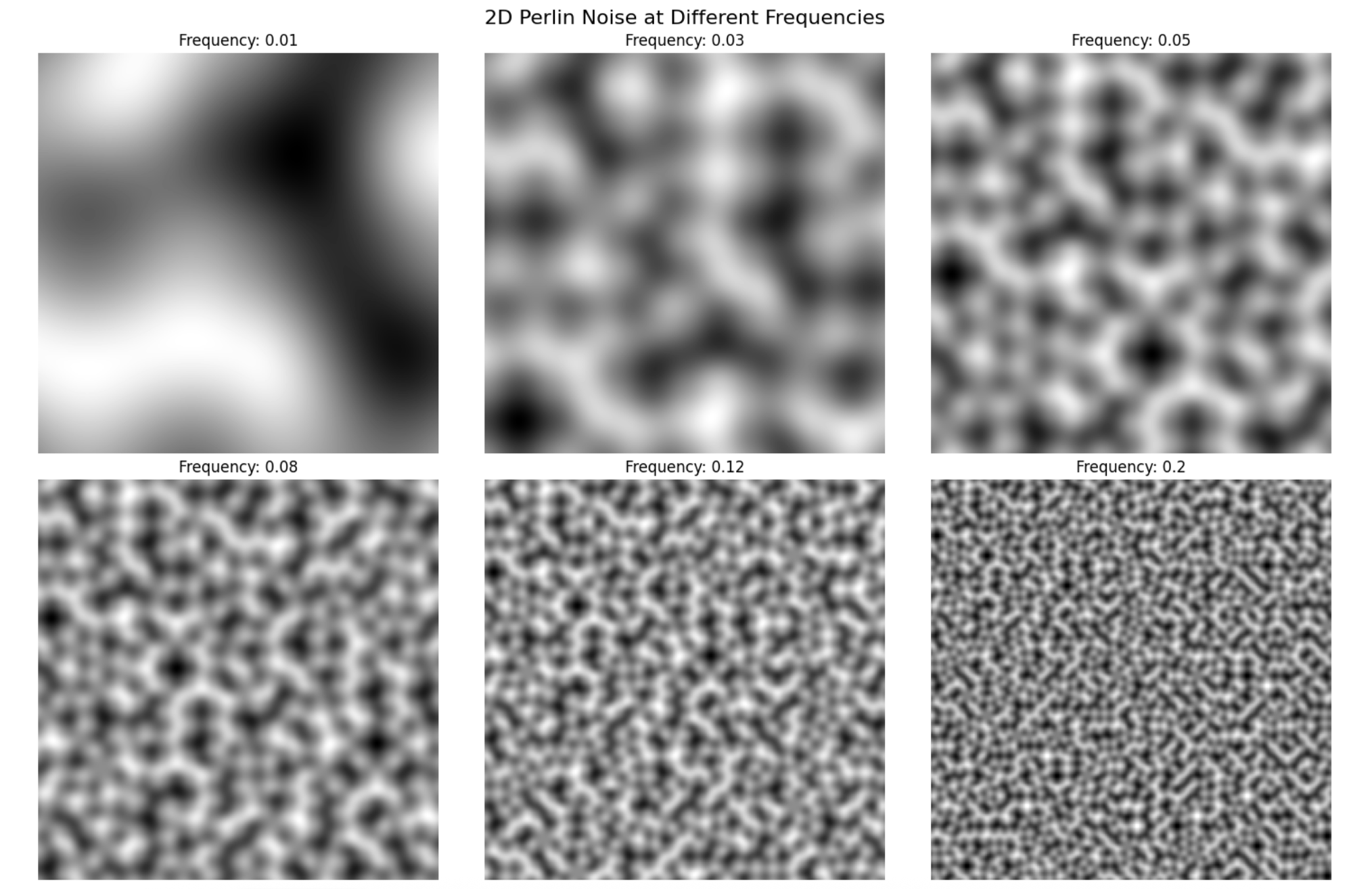
When inputs are integers, Perlin noise returns 0! This is because the vector from a grid point to itself is (0,0), and the dot product is 0.
Fractal Brownian Motion
Single-octave Perlin noise looks too smooth for most natural phenomena. So we use FBM that combines multiple octaves at different frequencies and amplitudes to create more realistic, detailed noise.
def fractal_brownian_motion(
    x: float, y: float, num_octaves: int = 6,
    frequency: float = 0.005, amplitude: float = 1.0,
    lacunarity: float = 2.0, persistence: float = 0.5) -> float:
    """
    Fractal Brownian Motion using multiple octaves of Perlin noise

    Args:
        x, y: Input coordinates
        num_octaves: Number of noise layers to combine
        frequency: Base frequency (how zoomed in the noise appears)
        amplitude: Base amplitude (how strong the effect is)
        lacunarity: Frequency multiplier between octaves (usually 2.0)
        persistence: Amplitude multiplier between octaves (usually 0.5)
    """

    result = 0.0
    current_amplitude = amplitude
    current_frequency = frequency

    for octave in range(num_octaves):
        # Calculate noise for this octave
        noise_val = noise_2d(
            x * current_frequency, y * current_frequency
        )

        # Add to result, weighted by current amplitude
        result += current_amplitude * noise_val

        # Prepare for next octave
        current_amplitude *= persistence
        current_frequency *= lacunarity

    return result
I have used this to create an Interactive Perlin Noise Explorer where you can control Frequency and octave sliders to see how noise is rendered on the grid!
This was super fascinating for me to explore that I made this game with the concepts from Perlin noise https://github.com/Sangarshanan/keep-walking Keep Walking is a browser-based 3D exploration game built with Procedural Terrain Generation using multiple layers of perlin noise (Made with claude code which super sped up my workflow)
// Base terrain with multiple octaves
const baseHeight = noise.octaveNoise(x, z, 6, 0.5, 0.008) * 32 +
                  noise.octaveNoise(x, z, 4, 0.3, 0.02) * 16;

// Add landscape features (mountains/valleys)
const finalHeight = applyLandscapeFeatures(x, z, baseHeight);
Check out the github repo with the link to the game and a lot more info about the game! If you are still here, congrats : ) you have a superior attention span.
Code is in this notebook along with an Interactive Perlin Noise Explorer
Links
- https://userpages.cs.umbc.edu/olano/s2002c36/ch04.pdf
- https://adrianb.io/2014/08/09/perlinnoise.html
- https://rtouti.github.io/graphics/perlin-noise-algorithm
- https://www.youtube.com/watch?v=CSa5O6knuwI
Leave a Comment